Klipsch Heresy IV Speaker Review

[Sal1950]

It is fricking trivial to build a high-sensitivity loudspeaker with very limited bandwidth and poor performance. It's not even hard to build one that's very efficient (i.e., skip the high-level crossover and go "fullrange"). I can do it in a half-hour with any of two dozen* "fullrange" drivers in the basement and a box. Such contrivances can be fun, but they're not hifi.

A ton of truth in what your saying.
OTOH, it was just as "fricking trivial" to design a speaker such as the highly revered LS3/5A .
A small speaker that has for it's time a relatively flat FR, but can't play loud, has loads of distortion if it
tries to do even slightly so, and no low bass. Also a "one trick pony."
Let the flames begin. LOL
I lived with my La Scala's for 32 years, and was well aware of their issues.
I tried to them improve them over that time with factory driver and crossover upgrades and tube amps.
But during all that time I never found anything that was in my budget that could replace them doing the things
that were a priority for my listening in those days.
Every speaker ever made was designed with it's own particular tradeoffs.
All things on balance the Heresy is and has been a "pretty good" little speaker.
JMHO YMMV

 

[Angsty]

but the proliferation of mods and improvements for the heritage Klipsch models speaks volumes (pun!) of the shortcomings of the factory products.

Not many models live to see seven decades of improvements.

 

[Rmar]

As always, I am copying/pasting from my website directly here. Therefore, some tables, pictures, paragraphs may look odd here. If you want to read the review from my site here is the link:
https://www.erinsaudiocorner.com/loudspeakers/klipsch_heresy_iv/

Link to YouTube review:

Klipsch Heresy IV Speaker Review

• Wednesday, Nov 25, 2020

View attachment 95822
Intro
The Klipsch Heresy IV is a 3-way speaker with a classic look. The Heresy IV features a 12-inch midwoofer, K-702 midrange compression driver, and K-704 Tractrix horn for high frequencies. On the back of the speaker is Klipsch’s new element to this speaker lineup: the Klipsch Tractrix port. This speaker can be bi-amped if desired thanks to the links on the two sets of terminals above the rear port. The Heresy IV comes in a variety of finishes and features a tweed grille to hide the drive units. The particular model I tested is the Cherry finish. Current retail for a pair is $3,000 USD.



I won’t get in to all the details of the speaker’s makeup as that can be found on the specification page here, or in the provided screenshot below. I would rather spend my time in this review discussing the performance.

View attachment 95824
BUT! I will provide some of my own photos…


View attachment 95825


View attachment 95827


View attachment 95828

View attachment 95829

Tweeter close-up:

View attachment 95830


Midrange close-up:

View attachment 95831



Speaker terminals:
View attachment 95832

Grille with the Klpsch Heresy logo:
View attachment 95826

Aesthetics are always a very personal thing. Some may not like the look of this speaker, but I do. I also fancy a lot of other designs that are more flashy. This speaker is the opposite of flashy, though, yet I still appreciate its retro aesthetic.

Objective Data
Unless otherwise noted, all the data below was captured using Klippel Distortion Analyzer 2 and Klippel modules (TRF, DIS, LPM, ISC to name a few). Most of the data was exported to a text file and then graphed using my own MATLAB scripts in order to present the data in a specific way I prefer. However, some is given using Klippel’s graphing.
Foreword: Subjective Analysis vs Objective Data (click for more)




Impedance Phase and Magnitude:
Impedance measurements are provided both at 0.10 volts RMS and 2.83 volts RMS. The low-level voltage version is standard because it ensures the speaker/driver is in linear operating range. The higher voltage is to see what happens when the output voltage is increased to the 2.83vRMS speaker sensitivity test.
View attachment 95833


View attachment 95834


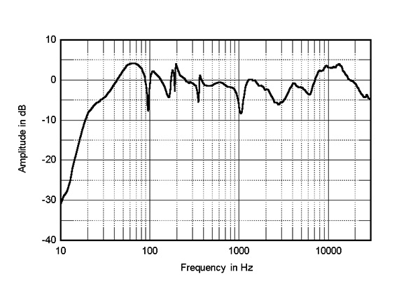
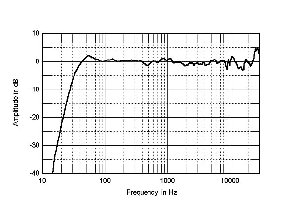
Frequency Response:

Notes about measurements (click for info)
The measurement below provides the frequency response at the reference measurement axis - also known as the 0-degree axis or “on axis” plane - in this measurement condition was situated at the tweeter. I did reach out to Klipsch directly - both via email and twitter - to ask what the designed reference axis was but received no reply. Per my research it seems everyone listens to these speakers on the tweeter axis (typical) so I proceeded with my measurements in that fashion.

The speaker was measured without the grille in place. I did not have the time to measure with the grille in place.
View attachment 95835

Below are both the horizontal and vertical response over a limited window (90° horizontal, ±40° vertical). I have provided a “normalized” set of data as well. The normalization simply means that I took the difference of the on-axis response and compared the other axes’ measurements to the on-axis response which gives the viewer a good idea of the speaker performance, relative to the on-axis response, as you move off-axis.

View attachment 95837


View attachment 95838

View attachment 95839

As I said above, the provided frequency response graphs were given with a limited set of data. I measured the response of the speaker’s vertical and horizontal axis in 10-degree steps over 360-degrees. Nearly 70 measurements in total are represented in my data. As you can imagine, providing all those data points in a single FR-type graphic below is a bit overwhelming and confusing for the viewer. A spectrogram is an alternate way to view this full set of data. This takes a 360-degree set of data and “collapses” it down to a rectangular representation of the various angles’ SPL. I have provided two sets of data: one set for horizontal and one for vertical. Each set consists of 2 graphics:

1. Full response (20Hz - 20kHz with the angles from 0° to ±180°) with absolute SPL values
2. Full, “normalized” response (20Hz - 20kHz with the angles from 0° to ±180°) with SPL values relative to the 0-degree axis

Normalized plots make it easier to compare how the speaker’s off-axis response behaves relative to the on-axis response curve.



View attachment 95841


View attachment 95842


View attachment 95843


View attachment 95844

The above spectrograms are the standard way of providing directivity graphics by most reviewers. Some prefer not to normalize the data. Some prefer to normalize the data. Either way, it’s a useful visual to get an idea of the directivity characteristics of a speaker or driver.
However, these “collapsed” representations of the sound field are not very intuitively viewed. At least not to me. So, I came up with a different way to view the speaker’s horizontal and vertical sound field by providing it across a 360° range in a globe plot below. I have provided both an absolute SPL version as well as a normalized version of both the horizontal and vertical sound fields.
Note the legend provided in the top left of each image which helps you understand speaker orientation provided in my global plots below.

View attachment 95845


View attachment 95846


View attachment 95847


View attachment 95848

Welp, I was interested in them for the aesthetic if nothing more, but there goes that idea.

CEA-2034 (aka: Spinorama):
The following set of data is populated via 360-degree, 10° stepped, “spins” from vertical and horizontal planes resulting in 70 unique measurements. Thus, this is sometimes referred to as “Spinorama” data. Audioholics has a great writeup on what these data mean (link here) and there is no sense in me trying to re-invent the wheel so I will reference you to them for further discussion. However, I will explain these curves lightly and provide my own spin on what they mean (pun totally intended). Sausalito Audio also has a good write-up on these curves here. Furthermore, you can find discussion in Dr. Floyd Toole’s book “Sound Reproduction”. Here is a great video of Dr. Toole discussing the use of measurements to quantify in-room performance.

In short, the CEA-2034 graphic below takes all the response measurements (horizontal and vertical) and applies weighting and averaging to sub-sets and can help provide an (accurate) prediction of the response in a typical room. If there is a single set of data to use in your purchase decision, this is probably it.
Alternatively, click this arrow, if you want my quick take on what these curves mean without going to another site.


View attachment 95849

Below is a breakout of the typical room’s Early Reflections contributors (floor bounce, ceiling, rear wall, front wall and side wall reflections). From this you can determine how much absorption you need and where to place it to help remedy strong dips from the reflection(s). In this case, the listening room would benefit from having at least a carpeted floor and, if willing to do so, acoustic absorption on the ceiling between the listener and the speakers.
View attachment 95850

And below is the Predicted In-Room response compared to a general target curve equaling -1dB/octave.

View attachment 95851
You may ask just how useful the above prediction is. Well, I’d be remiss for not delving in to that a little bit here. Please see my Analysis section below for discussion on this.


Harmonic Distortion:
Measurements were conducted at 2 meters ground plane using Klippel’s TRF module. Multiple output levels were tested to provide the trend of distortion component profiles and to provide a comparison against other drive units I have tested. The SPL provided is relative to 1 meter distance, averaged in the noted bandpass region.

View attachment 95852




Maximum Long Term SPL:
The below data provides the metrics for how Maximum Long Term SPL is determined. This measurement follows the IEC 60268-21 Long Term SPL protocol, per Klippel’s template, as such:

• Rated maximum sound pressure according IEC 60268-21 §18.4
• Using broadband multi-tone stimulus according §8.4
• Stimulus time = 60 s Excitation time + Preloops according §18.4.1

Each voltage test is 1 minute long (hence, the “Long Term” nomenclature).
The thresholds to determine the maximum SPL are:

• -20dB Distortion relative to the fundamental
• -3dB compression relative to the reference (1V) measurement

When the speaker has reached either or both of the above thresholds, the test is terminated and the SPL of the last test is the maximum SPL. In the below results I provide the summarized table as well as the data showing how/why this SPL was deemed to be the maximum.
This measurement is conducted once with a 20Hz to 20kHz multitone stimulus.
You can watch a demonstration of this testing via my YouTube channel:

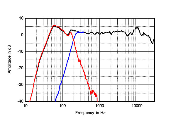
Test 1: 20Hz to 20kHz
Multitone compression testing. The red line shows the final measurement where either distortion and/or compression failed. The voltage just before this is used to help determine the maximum SPL.

View attachment 95853
Multitone distortion testing. The dashed blue line represents the -20dB (10% distortion) threshold for failure. The dashed red line is for reference and shows the 1% distortion mark (but has no bearing on pass/fail). The green line shows the final measurement where either distortion and/or compression failed. The voltage just before this is used to help determine the maximum SPL.

View attachment 95854





The above data can be summed up by:

• Max SPL for 20Hz to 20kHz is approximately 110dB @ 1 meter. The compression threshold was exceeded above this SPL.

 

[Rmar]

1. Hoffman's Iron Law. (Anton Hoffman having been the "H" in KLH)bt
2. There's no replacement for displacement.

It is fricking trivial to build a high-sensitivity loudspeaker with very limited bandwidth and poor performance. It's not even hard to build one that's very efficient (i.e., skip the high-level crossover and go "fullrange"). I can do it in a half-hour with any of two dozen* "fullrange" drivers in the basement and a box. Such contrivances can be fun, but they're not hifi.

It's not difficult even to build a multi-way loudspeaker system that'll scream up a storm within limited bandwidth and with compromised performance.
That's pretty much what the Heresy is -- or at was in its first two, if not three, iterations. It's a shrunken Cornwall and it sounds the part. I have no doubt that the fourth generation Heresy is better. I don't think it could be worse without actively trying to make it worse.

The heritage Klipsch get bashed because they're bright, harsh, aggressive sounding loudspeakers. The K-horn was OK, and actually the Cornwall does a pretty good job of sensitivity, dynamics, and LF extension -- but the proliferation of mods and improvements for the heritage Klipsch models speaks volumes (pun!) of the shortcomings of the factory products.

EDIT: In fairness, Altec was their own worst enemy when it came to crossover design and implementation.
... but boy howdy did they make some fine drivers and horns.

_________________
* Probably more than two dozen.

Most people are not setting their Heresy IV's them up correctly if they are harsh. With these bright horns, you have to have your listening position just south of the intersection of the left and right speakers. If, like most folks tend to do, you sit right in the cross-hairs, they will be harsh. Move your chair back 2 feet and you will have found nirvana.

 

[Rmar]

With horns, placement may be different that what many folks are used to with conventional drivers. For starters, put them as close as you can to either the corners, or to the side walls leaving about 12". This next part is even more critical. Place you primary listening position at about two (2) foot behind the axis. Or conversely, if you can't move your chair, then toe the Heresey IV's in some more until the axis is 2 foot in front of you. In the manual it says to "angle speakers towards the listener" and then "experient" with the guidelines. The diagram in the book is wrong, or you could say it is the "pre-experient" position. Experienced Heresy owners know that the book is not correct.No one would have their horn speakers aiming right at the ears. That's tantamount to holding a fog horn to your head and blasting it. Move your chair back from the axis and you will open up an entirely new Heresy IV experience for yourself. It will be the experience that you have heard about and the reason why this speaker has sold strong for five decades. You will know why people use words like "Amazing, huge sound stage, holographic, stunning..." and on and on. You knew there had to be some reason folks loved them!

It is unfortunate this young fellow spent all that time doing his charts and graphs with a set up that was sub-optimal. It is also too bad for Klipsch, because when people pass off "science" as gospel, and when that "science" is based on the wrong assumptions or the wrong test set-up, it misleads others. All trained scientists know that before they start testing, they are required to "review the literature," to find out what others know, before they jump to hypothesis making or testing. Finding out what others know about the Heresy seems to have been missed in this case.

Lastly, if newcomers to the Heresy IV are interested, there is another tip they may be interested in. And that is to wrap Dynamat around the squawker. The squaker is the middle speaker. That will make a wonderful speaker even better.

 

[Sal1950]

It is unfortunate this young fellow spent all that time doing his charts and graphs with a set up that was sub-optimal. It is also too bad for Klipsch, because when people pass off "science" as gospel, and when that "science" is based on the wrong assumptions or the wrong test set-up, it misleads others. All trained scientists know that before they start testing, they are required to "review the literature," to find out what others know, before they jump to hypothesis making or testing.

I can appreciate your support of the Heresy's, like many speakers they have some strong points and some
weak points. As a 32y owner of La Scala's I'm intimately aware of most of them.
I'll agree the last thing you want to do is listen directly on axis and I also found the best setup for imaging to be crossing
over a bit in front of the listeners head.
That said, your criticism of Erin's review and measurements is quite in error. His measurements using the Klippel system
do reveal everything the Heresy is capable of both on and off axis. The fact is that all the speakers in the Heritage line have
very bad irregularities in frequency response no matter how you position them that could only be very slightly moderated by set-up.
A possible better approach might be to use a good DRC system to smooth the response a bit.

 

[mhardy6647]

 

[Sal1950]

What are the large square boxes in front with the small monitors sitting on top, Altec's?

 

[mhardy6647]

Yes, Santiagos.
They have very little cred with the Altecistas, but they sound pretty good to me. For a variety of reasons, I kept them instead of the Valencias I had, in fact.
That said, their primary use nowadays is as speaker stands.

 

[Sal1950]

Yes, Santiagos.
They have very little cred with the Altecistas, but they sound pretty good to me. For a variety of reasons, I kept them instead of the Valencias I had, in fact.

Very kool. thanks for the response.
Every time I see you post a photo of your room I turn green with jealousy.
What a perfect frickin space to set-up and tune a Hi-Fi plus extras!
Enjoy

 

[Rmar]

I can appreciate your support of the Heresy's, like many speakers they have some strong points and some
weak points. As a 32y owner of La Scala's I'm intimately aware of most of them.
I'll agree the last thing you want to do is listen directly on axis and I also found the best setup for imaging to be crossing
over a bit in front of the listeners head.
That said, your criticism of Erin's review and measurements is quite in error. His measurements using the Klippel system
do reveal everything the Heresy is capable of both on and off axis. The fact is that all the speakers in the Heritage line have
very bad irregularities in frequency response no matter how you position them that could only be very slightly moderated by set-up.
A possible better approach might be to use a good DRC system to smooth the response a bit.

I can appreciate your support of the Heresy's, like many speakers they have some strong points and some
weak points. As a 32y owner of La Scala's I'm intimately aware of most of them.
I'll agree the last thing you want to do is listen directly on axis and I also found the best setup for imaging to be crossing
over a bit in front of the listeners head.
That said, your criticism of Erin's review and measurements is quite in error. His measurements using the Klippel system
do reveal everything the Heresy is capable of both on and off axis. The fact is that all the speakers in the Heritage line have
very bad irregularities in frequency response no matter how you position them that could only be very slightly moderated by set-up.
A possible better approach might be to use a good DRC system to smooth the response a bit.

I am defending science. Nothing else. This is "Audio Science Review." If present your work as science, then make sure it is and not a method to get folks to click your links for personal profit. That's not science, my friend. That said, your criticism of me is quiet in error.

 

[Angsty]

I can appreciate your support of the Heresy's, like many speakers they have some strong points and some
weak points. As a 32y owner of La Scala's I'm intimately aware of most of them.
I'll agree the last thing you want to do is listen directly on axis and I also found the best setup for imaging to be crossing
over a bit in front of the listeners head.
That said, your criticism of Erin's review and measurements is quite in error. His measurements using the Klippel system
do reveal everything the Heresy is capable of both on and off axis. The fact is that all the speakers in the Heritage line have
very bad irregularities in frequency response no matter how you position them that could only be very slightly moderated by set-up.
A possible better approach might be to use a good DRC system to smooth the response a bit.

I agree with @Sal1950 regarding the Heresy measurements. I’m unclear why @Rmar believes they are flawed.

 

[rynberg]

It is unfortunate this young fellow spent all that time doing his charts and graphs with a set up that was sub-optimal. It is also too bad for Klipsch, because when people pass off "science" as gospel, and when that "science" is based on the wrong assumptions or the wrong test set-up, it misleads others. All trained scientists know that before they start testing, they are required to "review the literature," to find out what others know, before they jump to hypothesis making or testing. Finding out what others know about the Heresy seems to have been missed in this case.

What a condescending and ignorant reply...you might want to start reading some audio reproduction science books while sitting in your glass house. Do you even know what a Klippel is?

 

[Rmar]

What if a high end speaker measures really badly?​

---

The problem with "objective" measurements is that do not tell you what the "objective" was. It's the fallacy of science. More than half of the best speakers in the world do not measure flat. Expert designers design speakers for specific sound experiences by the listener, not to achieve a flat speaker response.

Folks that only focus on a "flat response" are those that want to sound smart and scientific when in fact they are the very ones that don't understand science. Numbers are meaningless unless you understand how to interpret them in their full context.

Cheap speakers makers love the "flat response crowd." To sell them speakers, all they have to do is get a flat response and this group will buy them. They buy them whether or not they sound good. As long is the curve is flat. Their ears will adjust and they will eventually learn to love them.

Use your brains, people! And not the numbers people push on you.


****************************************************************************************************
What smart people say.....starting below.


You know, it's true that I feel listening is more important than measurements and that it's generally difficult to really tie together measurements with pleasure. Below 0.05% THD do I care? No I do not. I really don't care. The number tells me nothing about whether I'd like the amp more or not anymore.
In this one memorable review for the Alta Audio Adam speaker, I really felt shivers go up my spine when I looked at the measurements, especially at ~$20kUSD. This looks like an absolute hot mess. Does it sound this bad though? I certainly don't have the $20K to test that out myself. What do you all think?

erik_squires04-24-2024 2:27pm

21 responses

• 
  

soix​ 8,644 posts 04-24-2024 at 03:30pm This is timely as there have been discussions of specifically the Alta Alyssa here recently. I was curious about the brand having heard good things so have read several reviews and comments from people who’ve heard Alta speakers at shows, and although there are some glowing comments there are also detractors citing things like frequency balance that can obviously be very room dependent and, more concerning, discontinuity between drivers. I’m like you in that I look at measurements and find them useful and helpful, but the final arbiter is always my my ears, but in this particular case I can’t help thinking the measurements are exposing issues that might actually be audible for some listeners. At the very least this would seem to indicate that Alta speakers, even more so than most other speakers, need to be auditioned in person and preferably in one’s own room if at all possible.

audiorusty​ 265 posts 04-24-2024 at 04:22pm I have never cared and highly likely I never will care how a speaker measures. For that matter I have never bothered to investigate how well a speaker measures. The only measurement I care about is how does it sound to me. If I can't audition a speaker I will not buy that speaker.

middlemass​ 873 posts 04-24-2024 at 04:41pm If it measures badly and sounds good, it is good. If it measures good and sounds bad, it is bad.

deep_333​ 762 posts 04-24-2024 at 05:27pm Hmmm, let me take a guess.... He a) bought the drivers from someone else b) threw it in a box in an exotic garage and c) wants to charge 20k for something that measures like this...meh No thanks...I’d probably send this speaker back to its daddy. (In general, put some high caliber electronics on any pig and it could start to sound pleasing at some point. But, the pig is still a pig that’s getting carried.) If a speaker costs 5k and above, my core requirements are: a) All drivers need to designed/developed in-house from scratch! b) Everything about the speaker should be designed from the ground up! c) Measurements should indicate engineering competence, even if it is not pristine Here are the measurements close to my 30k speaker (everything developed in-house from scratch by the manufacturer) Here’s the measurement on my 15k speaker (everything developed in-house from scratch by the manufacturer) Here’s the measurement on my 5k speaker (everything developed in-house from scratch by the manufacturer) If it is under 5k, i am forgiving of the drivers coming from someone else. I’ll forgive you!! But, now, it better measure like a pristine cat, because the manufacturer’s doing way less work now!! So, here’s my 3k speaker (~1500 if ya DIY’d the kit) with drivers from someone else.

audiokinesis​ 2,713 posts 04-24-2024 at 05:32pm Narrow-band peaks and dips which occur within about 1/3 octave of one another tend to be "averaged" by the ear. Therefore, that on-axis frequency response graph looks far worse to the eyes than it sounds to the ears. The on-axis dip at 3 kHz is wide enough to survive the ear's "averaging" characteristic, BUT it corresponds with an off-axis rise in that region. So my guess is the designer put a dip at the bottom end of the tweeter’s range to compensate for an off-axis "flare". Imo this is a good design choice. The on-axis emphasis centered around 11 kHz can be compensated for by listening off-axis. In fact, it looks to me like at about maybe 10-20 degrees off-axis the 3 kHz dip fills in and the 11 kHz bump smooths out. My guess is that this speaker would sound excellent with proper set-up. Duke Not an Alta Audio dealer

csmgolf​ 871 posts 04-24-2024 at 05:34pm @soix has it right. The Alta Audio speakers should be listened to before buying. I was one of those commenting on the Alyssa thread about frequency response and discontinuity issues. There were three speakers from them represented at Axpona. I heard the same issue on all of them. After the show, I wanted to see if there were measurements out there showing what I heard. Stereophile measurements of the Adam and Alyssa clearly show issues at around 3k, and to me it is audible. I wanted to like them, because they look beautiful. Some people may like the sound that they produce, I did not.

sounds_real_audio​ 944 posts 04-24-2024 at 06:16pm Well then it better sound good.

jond​ 5,660 posts 04-24-2024 at 07:41pm I turned my laptop speakers up all the way and I still can't hear that graph. So no comment.

mapman​ 21,835 posts 04-24-2024 at 08:17pm Probably not myself personally, but If someone likes the sound of an expensive speaker it does not matter that it does not measure well or technically may be poorly designed or implemented. The off base measurements will probably be an indicator of the particular unique sound that is liked and is less likely to be found elsewhere. In other words a poorly engineered speaker may sound unique and distinguish itself from others but the reason it sounds that way may not be a very good one. Or one may just be drawn to a product by aesthetics. You have to live with your speakers so looks matter. It’s all good even if not so much technically.

helomech​ 1,494 posts 04-24-2024 at 08:44pm If it measures “really badly,” then it’s not a high end speaker IME. All the absolute best speakers I’ve heard and owned measure exceptionally well. I have zero doubt that these days I would be able to quickly hear the issues with that Alta speaker. A decade ago when I was much less experienced, it’s likely that had I auditioned that same speaker, I would’ve thought it pretty good.

mapman​ 21,835 posts 04-24-2024 at 08:58pm Seems to me the correlation between high end and cost is much higher than the correlation between high end and measured sound quality.

erik_squires OP​ 15,647 posts 04-24-2024 at 09:43pm The Alta Alyssa also seems to be radically oddly designed. In the case of the Adam it's almost as if the designers have deliberately introduced some comb filtering into the frequency response, kind of a hard thing to do if you are paying even moderate attention in crossover theory class. Perhaps the radically different response curves make the speakers sound more detailed and make the reviewer go through their entire album collection again to hear what they've been missing.... Sorry, that's a bit of a cliche I read when speakers are deliberately ragged. If the peaks and dips are not audible, as @audiokinesis suggests then I wonder why and how they went through all the trouble to introduce them in the first place?

helomech​ 1,494 posts 04-24-2024 at 09:51pm If it measures badly and sounds good, it is good. If it measures good and sounds bad, it is bad. Wow, what incredible and original insight! Haven’t heard that one before.

audiokinesis​ 2,713 posts 04-24-2024 at 10:14pm @erik_squires wrote: "If the peaks and dips are not audible, as @audiokinesis suggests then I wonder why and how they went through all the trouble to introduce them in the first place?" I think the up/down peak/dip jogs are artifacts of the enclosure design, which is apparently a transmission line/port hybrid. There are corresponding little spikes in the impedance curve that look like what I've seen in some of my transmission line builds.

2psyop​ 1,501 posts 04-24-2024 at 10:29pm I have yet to hear anyone listen to measurements when listening to a pair of speakers, therefore I really don't pay attention to them....

mapman​ 21,835 posts 04-24-2024 at 10:48pm Fwiw I have kef ls50 meta ( + Klipsch sw308 powered sub), Ohm Walsh and Sonus Faber Concerto Domus each in different rooms. I use Roon DSP to tweak the sound of each in their corresponding rooms. The KEFs are known for their good technical measurements. The Sonus Faber also have measured well but not as well as the KEFs. I have seen measurements of earlier Ohm Walsh models from years ago and they tend to be good but are not as conclusive perhaps due to age. Each room’s acoustics measure much differently and each has its rougher areas that I have tackled via room correction using Roon DSP. These are all “good quality” speakers. Once room is corrected for they start to sound more similar than different in regards to tonality. Soundstage imaging and detail is very good in each case but each is somewhat unique in this regard. So once room is corrected I then use Parametric EQ in Roon DSP to tailor to my taste. The good measuring kefs require the least, just a bit of a bump from 4-6khz to liven things up a tad. The other two may get a similar bump but there are also remaining high end and bass related tweaks I apply to get them sounding just right to me at my listening position. So after all that in the end they each sound quite similar in regards to tone. The kefs are the ones that reveal the most detail in the recordings. The Sonus Faber provide a touch of added “musicality” that I would attribute to their cabinet designed to deliver sound more like an orchestral string instrument. The pseudo-Omnidirectional Ohms are somewhere in between and always excel at delivering a live like sound where the players are in your room as opposed to you being drawn into the recording. So there you have it. Measures serve a purpose to help differentiate gear out of the box and also facilitate getting them tweaked effectively as needed but alone do not assure a clear winner. No surprise there eh? Also I have learned that DSP is the great equalizer. No reason these days to be stuck with the sound you get out of the box. If the speakers are up to the task given the room at hand, almost anything is possible from there with a proper amp and DSP.

asvjerry​ 4,264 posts 04-24-2024 at 10:58pm Sometimes, it's the charts/graphs/measured specs that catch the eye and make the ears desire a listen of.... But having to explore and posit what v. why to such a degree makes this mortal consider that make these 'A' series units seem to be 'space finicky'... You wouldn't know if you Really Like them until in Your space with them. At 20K$-ish, one might be tempted to look about at 'other items in place' and enter into the old '...what if it's the....?' hunter/gatherer routine.... No dog in the hunt (and no $ to join in, either), I'd keep shopping. Don't need more complications in a life with enough already.... A 195hz 'dip' due to the enclosures' back panel...Occam's Razor, anyone?

laoman​ 358 posts 04-24-2024 at 11:08pm Measurements are not important; it is how the equipment sounds to you that matters.

mapman​ 21,835 posts 04-24-2024 at 11:28pm I’ll go out on a limb and assert that in the end, proper application of measurements always helps to achieve one’s hifi sound goals faster, more effectively and for less. The trick is to be able to understand and apply the numbers properly and I think that is not easy but a worthwhile goal for any audiophile. More good and reliable data informs better decision making. But the devil is always in the details. Practically though, each will end up finding their own way as best they can. Sometimes it’s the journey that matters more than reaching the final destination. It’s all good. Cheers!

wolf_garcia​ 6,600 posts 04-25-2024 at 03:31am Efficiency is important to me as one of my amps (a class tube A SEP) has relatively low power...impedance is important, but the sound is really all that matters...and I'll never buy anything without auditioning unless it has a very fair return policy.

yoyoyaya​ 601 posts 04-25-2024 at 05:54am @erik_squires - that's a very ragged frequency response graph. I don't think speakers have to measure perfectly to sound good - Wilson Audio speakers are not textbook. But there's a difference between small deviations and big ones.

Log in to respond

More to discover​

• Cartridge Compliance Measures
• What if a high end speaker measures r...
• Stereophile & Mytek Brooklyn - Be...

NTT Audio Lab 103​

TAD TAD Micro Evolution ME1​

ATC SCM40 ​

© 2024 Audiogon.com

• Contact Us
• Help
• Terms of Use
• Guidelines

 

[Rmar]

I agree with @Sal1950 regarding the Heresy measurements. I’m unclear why @Rmar believes they are flawed.

 

[levimax]

It's the fallacy of science. Wake up folks. You are being mislead by the marketing departments of many companies.

Not sure if you are trolling or really don't understand the speaker measurements presented here. Flat on axis reponse is one measurement of many presented. You need to look at all the measurements together to understand a speakers strengths and weaknesses.

 

[bodhi]

I think this will be resolved in that another thread.

 

[Everett T]

I am defending science. Nothing else. This is "Audio Science Review." If present your work as science, then make sure it is and not a method to get folks to click your links for personal profit. That's not science, my friend. That said, your criticism of me is quiet in error.

What isn't scientific about the measurement analysis from the Klippel NFS? The interpretation of that data could be flawed in the written, but the data is the data.

As for affiliate links, that helps offset the time and costs associated with each measurement and the equipment. Same as donations here at ASR. Erin's day job at NASA puts the food in the table and cares for his children. If you're gonna complain about Erin, the likes of Stereophile, Hometheater Fidelity, etc, where they're completely dependent on adv dollars, would be a more realistic "target".

 

[Everett T]

What if a high end speaker measures really badly?​

---

The problem with "objective" measurements is that do not tell you what the "objective" was. It's the fallacy of science. More than half of the best speakers in the world do not measure flat. Expert designers design speakers for specific sound experiences by the listener, not to achieve a flat speaker response.

Folks that only focus on a "flat response" are those that want to sound smart and scientific when in fact they are the very ones that don't understand science. Numbers are meaningless unless you understand how to interpret them in their full context.

Cheap speakers makers love the "flat response crowd." To sell them speakers, all they have to do is get a flat response and this group will buy them. They buy them whether or not they sound good. As long is the curve is flat. Their ears will adjust and they will eventually learn to love them.

Use your brains, people! And not the numbers people push on you.


****************************************************************************************************
What smart people say.....starting below.


You know, it's true that I feel listening is more important than measurements and that it's generally difficult to really tie together measurements with pleasure. Below 0.05% THD do I care? No I do not. I really don't care. The number tells me nothing about whether I'd like the amp more or not anymore.
In this one memorable review for the Alta Audio Adam speaker, I really felt shivers go up my spine when I looked at the measurements, especially at ~$20kUSD. This looks like an absolute hot mess. Does it sound this bad though? I certainly don't have the $20K to test that out myself. What do you all think?

erik_squires04-24-2024 2:27pm

21 responses

• 
  
• 
  

soix​ 8,644 posts 04-24-2024 at 03:30pm This is timely as there have been discussions of specifically the Alta Alyssa here recently. I was curious about the brand having heard good things so have read several reviews and comments from people who’ve heard Alta speakers at shows, and although there are some glowing comments there are also detractors citing things like frequency balance that can obviously be very room dependent and, more concerning, discontinuity between drivers. I’m like you in that I look at measurements and find them useful and helpful, but the final arbiter is always my my ears, but in this particular case I can’t help thinking the measurements are exposing issues that might actually be audible for some listeners. At the very least this would seem to indicate that Alta speakers, even more so than most other speakers, need to be auditioned in person and preferably in one’s own room if at all possible.

audiorusty​ 265 posts 04-24-2024 at 04:22pm I have never cared and highly likely I never will care how a speaker measures. For that matter I have never bothered to investigate how well a speaker measures. The only measurement I care about is how does it sound to me. If I can't audition a speaker I will not buy that speaker.

middlemass​ 873 posts 04-24-2024 at 04:41pm If it measures badly and sounds good, it is good. If it measures good and sounds bad, it is bad.

deep_333​ 762 posts 04-24-2024 at 05:27pm Hmmm, let me take a guess.... He a) bought the drivers from someone else b) threw it in a box in an exotic garage and c) wants to charge 20k for something that measures like this...meh No thanks...I’d probably send this speaker back to its daddy. (In general, put some high caliber electronics on any pig and it could start to sound pleasing at some point. But, the pig is still a pig that’s getting carried.) If a speaker costs 5k and above, my core requirements are: a) All drivers need to designed/developed in-house from scratch! b) Everything about the speaker should be designed from the ground up! c) Measurements should indicate engineering competence, even if it is not pristine Here are the measurements close to my 30k speaker (everything developed in-house from scratch by the manufacturer) Here’s the measurement on my 15k speaker (everything developed in-house from scratch by the manufacturer) Here’s the measurement on my 5k speaker (everything developed in-house from scratch by the manufacturer) If it is under 5k, i am forgiving of the drivers coming from someone else. I’ll forgive you!! But, now, it better measure like a pristine cat, because the manufacturer’s doing way less work now!! So, here’s my 3k speaker (~1500 if ya DIY’d the kit) with drivers from someone else.

audiokinesis​ 2,713 posts 04-24-2024 at 05:32pm Narrow-band peaks and dips which occur within about 1/3 octave of one another tend to be "averaged" by the ear. Therefore, that on-axis frequency response graph looks far worse to the eyes than it sounds to the ears. The on-axis dip at 3 kHz is wide enough to survive the ear's "averaging" characteristic, BUT it corresponds with an off-axis rise in that region. So my guess is the designer put a dip at the bottom end of the tweeter’s range to compensate for an off-axis "flare". Imo this is a good design choice. The on-axis emphasis centered around 11 kHz can be compensated for by listening off-axis. In fact, it looks to me like at about maybe 10-20 degrees off-axis the 3 kHz dip fills in and the 11 kHz bump smooths out. My guess is that this speaker would sound excellent with proper set-up. Duke Not an Alta Audio dealer

csmgolf​ 871 posts 04-24-2024 at 05:34pm @soix has it right. The Alta Audio speakers should be listened to before buying. I was one of those commenting on the Alyssa thread about frequency response and discontinuity issues. There were three speakers from them represented at Axpona. I heard the same issue on all of them. After the show, I wanted to see if there were measurements out there showing what I heard. Stereophile measurements of the Adam and Alyssa clearly show issues at around 3k, and to me it is audible. I wanted to like them, because they look beautiful. Some people may like the sound that they produce, I did not.

sounds_real_audio​ 944 posts 04-24-2024 at 06:16pm Well then it better sound good.

jond​ 5,660 posts 04-24-2024 at 07:41pm I turned my laptop speakers up all the way and I still can't hear that graph. So no comment.

mapman​ 21,835 posts 04-24-2024 at 08:17pm Probably not myself personally, but If someone likes the sound of an expensive speaker it does not matter that it does not measure well or technically may be poorly designed or implemented. The off base measurements will probably be an indicator of the particular unique sound that is liked and is less likely to be found elsewhere. In other words a poorly engineered speaker may sound unique and distinguish itself from others but the reason it sounds that way may not be a very good one. Or one may just be drawn to a product by aesthetics. You have to live with your speakers so looks matter. It’s all good even if not so much technically.

helomech​ 1,494 posts 04-24-2024 at 08:44pm If it measures “really badly,” then it’s not a high end speaker IME. All the absolute best speakers I’ve heard and owned measure exceptionally well. I have zero doubt that these days I would be able to quickly hear the issues with that Alta speaker. A decade ago when I was much less experienced, it’s likely that had I auditioned that same speaker, I would’ve thought it pretty good.

mapman​ 21,835 posts 04-24-2024 at 08:58pm Seems to me the correlation between high end and cost is much higher than the correlation between high end and measured sound quality.

erik_squires OP​ 15,647 posts 04-24-2024 at 09:43pm The Alta Alyssa also seems to be radically oddly designed. In the case of the Adam it's almost as if the designers have deliberately introduced some comb filtering into the frequency response, kind of a hard thing to do if you are paying even moderate attention in crossover theory class. Perhaps the radically different response curves make the speakers sound more detailed and make the reviewer go through their entire album collection again to hear what they've been missing.... Sorry, that's a bit of a cliche I read when speakers are deliberately ragged. If the peaks and dips are not audible, as @audiokinesis suggests then I wonder why and how they went through all the trouble to introduce them in the first place?

helomech​ 1,494 posts 04-24-2024 at 09:51pm Wow, what incredible and original insight! Haven’t heard that one before.

audiokinesis​ 2,713 posts 04-24-2024 at 10:14pm @erik_squires wrote: "If the peaks and dips are not audible, as @audiokinesis suggests then I wonder why and how they went through all the trouble to introduce them in the first place?" I think the up/down peak/dip jogs are artifacts of the enclosure design, which is apparently a transmission line/port hybrid. There are corresponding little spikes in the impedance curve that look like what I've seen in some of my transmission line builds.

2psyop​ 1,501 posts 04-24-2024 at 10:29pm I have yet to hear anyone listen to measurements when listening to a pair of speakers, therefore I really don't pay attention to them....

mapman​ 21,835 posts 04-24-2024 at 10:48pm Fwiw I have kef ls50 meta ( + Klipsch sw308 powered sub), Ohm Walsh and Sonus Faber Concerto Domus each in different rooms. I use Roon DSP to tweak the sound of each in their corresponding rooms. The KEFs are known for their good technical measurements. The Sonus Faber also have measured well but not as well as the KEFs. I have seen measurements of earlier Ohm Walsh models from years ago and they tend to be good but are not as conclusive perhaps due to age. Each room’s acoustics measure much differently and each has its rougher areas that I have tackled via room correction using Roon DSP. These are all “good quality” speakers. Once room is corrected for they start to sound more similar than different in regards to tonality. Soundstage imaging and detail is very good in each case but each is somewhat unique in this regard. So once room is corrected I then use Parametric EQ in Roon DSP to tailor to my taste. The good measuring kefs require the least, just a bit of a bump from 4-6khz to liven things up a tad. The other two may get a similar bump but there are also remaining high end and bass related tweaks I apply to get them sounding just right to me at my listening position. So after all that in the end they each sound quite similar in regards to tone. The kefs are the ones that reveal the most detail in the recordings. The Sonus Faber provide a touch of added “musicality” that I would attribute to their cabinet designed to deliver sound more like an orchestral string instrument. The pseudo-Omnidirectional Ohms are somewhere in between and always excel at delivering a live like sound where the players are in your room as opposed to you being drawn into the recording. So there you have it. Measures serve a purpose to help differentiate gear out of the box and also facilitate getting them tweaked effectively as needed but alone do not assure a clear winner. No surprise there eh? Also I have learned that DSP is the great equalizer. No reason these days to be stuck with the sound you get out of the box. If the speakers are up to the task given the room at hand, almost anything is possible from there with a proper amp and DSP.

asvjerry​ 4,264 posts 04-24-2024 at 10:58pm Sometimes, it's the charts/graphs/measured specs that catch the eye and make the ears desire a listen of.... But having to explore and posit what v. why to such a degree makes this mortal consider that make these 'A' series units seem to be 'space finicky'... You wouldn't know if you Really Like them until in Your space with them. At 20K$-ish, one might be tempted to look about at 'other items in place' and enter into the old '...what if it's the....?' hunter/gatherer routine.... No dog in the hunt (and no $ to join in, either), I'd keep shopping. Don't need more complications in a life with enough already.... A 195hz 'dip' due to the enclosures' back panel...Occam's Razor, anyone?

laoman​ 358 posts 04-24-2024 at 11:08pm Measurements are not important; it is how the equipment sounds to you that matters.

mapman​ 21,835 posts 04-24-2024 at 11:28pm I’ll go out on a limb and assert that in the end, proper application of measurements always helps to achieve one’s hifi sound goals faster, more effectively and for less. The trick is to be able to understand and apply the numbers properly and I think that is not easy but a worthwhile goal for any audiophile. More good and reliable data informs better decision making. But the devil is always in the details. Practically though, each will end up finding their own way as best they can. Sometimes it’s the journey that matters more than reaching the final destination. It’s all good. Cheers!

wolf_garcia​ 6,600 posts 04-25-2024 at 03:31am Efficiency is important to me as one of my amps (a class tube A SEP) has relatively low power...impedance is important, but the sound is really all that matters...and I'll never buy anything without auditioning unless it has a very fair return policy.

yoyoyaya​ 601 posts 04-25-2024 at 05:54am @erik_squires - that's a very ragged frequency response graph. I don't think speakers have to measure perfectly to sound good - Wilson Audio speakers are not textbook. But there's a difference between small deviations and big ones.

Log in to respond

More to discover​

• Cartridge Compliance Measures
• What if a high end speaker measures r...
• Stereophile & Mytek Brooklyn - Be...

NTT Audio Lab 103​

TAD TAD Micro Evolution ME1​

ATC SCM40 ​

© 2024 Audiogon.com

• Contact Us
• Help
• Terms of Use
• Guidelines

You complain that people only look for flat responses and yet you only show frequency plots to form your opinion, not the full set of measurements. Yes, many focus on just the on axis response, so what when the entire data set is available for evaluation? The reviewers I know attempt to correlate the data they see into what they hear, if it is audible, they note it.

It's sounds like you have things backwards, where the data isn't the most valuable tool we have for pre-evaluation and where the reviewers subjective opinion is more important...

Edit: As for drivers, it doesn't matter whether it's made in house or sourced, as that is not an indication of a good driver.

 

[Rmar]

I like data measurements as much as the next guy, but as a forum with "science" as its middle name, the amount of "not-science" written into this review is shocking. The over generalizations, the personal beliefs and opinions; and the ad hominem style categorizations in the "conclusion" are juvenile.

"These are not an accurate speaker. I do not believe others expect that to be the case. I just want to make that clear up front. They may very well play your favorite rock n’ roll album with the zest you love, but they are not a reference speaker. Their response is too unbalanced for that task (both subjectively and certainly objectively). In my opinion, these are party speakers. They are show-off speakers when your neighbor comes over bragging about his Bose setup. The Heresy IV is what I would call a Jekyll/Hyde speaker. Sometimes they make your music fun and sometimes they make it boring. Heck, sometimes they make it aggravating. It’s a grab bag depending on what track you come across and your mood at the time."

If we are going to have a scientific, data-driven review of equipment, let's stick to the expected standards from beginning to end. Save the silly commentary for happy-hour.

The quote above was from the review. Does that sound like a scientific conclusion based on scientific test and measurement? If it does, then you are also the type that is very willing to spend $100.00 dollars on a nice dinner out with your wife, choosing the newest item on the menu, even after the waitress let you know it had only been tested one time buy a guy on the floor of his garage. Enjoy your meal!